Tutorial - Part #1 - The SingleImage Class

In this first tutorial the basics of the methods and properties of the SingleImage class are explained.

This object class represents the basic unit of data which we will manipulate. Basically it starts containing pixel data, with its mask. First lets create an instance of this class with a numpy array.

import numpy as np
import matplotlib.pyplot as plt

from properimage import single_image as s

%matplotlib inline

pixel = np.random.random((128,128))*5.
# Add some stars to it
star = [[35, 38, 35],
        [38, 90, 39],
        [35, 39, 34]]
for i in range(25):
    x, y = np.random.randint(120, size=2)
    pixel[x:x+3,y:y+3] = star

mask = np.random.randint(2, size=(128,128))
for i in range(10):
    mask = mask & np.random.randint(2, size=(128,128))

img  = s.SingleImage(pixel, mask)

We can see that the img object created automatically produces an output displaying the number of sources found.

This just accounts for sources good enough for PSF estimation, which is the first step for any processing ProperImage is intended for.

If we try to print the instance, (or obtain the representation output) we find that the explicit origin of the data is being displayed

print(img)

SingleImage instance for ndarray

If you would like to acces the data inside the object img just ask for data.

img.data

masked_array(
  data=[[4.05117654800415, 2.3367366790771484, 3.358428478240967, ...,
         2.9861879348754883, 2.9639270305633545, 2.42071795463562],
        [0.7913976907730103, 0.396319717168808, 4.990025997161865, ...,
         2.640835762023926, 0.19548970460891724, 4.581973075866699],
        [0.21659301221370697, 3.309115409851074, 3.2671613693237305, ...,
         0.602097749710083, 1.2853821516036987, 4.894009113311768],
        ...,
        [3.6120381355285645, 0.2359519749879837, 4.402842998504639, ...,
         3.145235300064087, 1.6198410987854004, 4.595581531524658],
        [1.655808687210083, 2.216202735900879, 2.922168254852295, ...,
         4.323221206665039, 4.086019515991211, 4.8711090087890625],
        [1.7609387636184692, 4.972808837890625, 2.632087469100952, ...,
         3.8503310680389404, 0.36555567383766174, 1.0644891262054443]],
  mask=[[False, False, False, ..., False, False, False],
        [False, False, False, ..., False, False, False],
        [False, False, False, ..., False, False, False],
        ...,
        [False, False, False, ..., False, False, False],
        [False, False, False, ..., False, False, False],
        [False, False, False, ..., False, False, False]],
  fill_value=1e+20,
  dtype=float32)

As can be seen it is a numpy masked array, with bad pixels flagged.

plt.figure(figsize=(6,6))
plt.imshow(img.data, cmap='Greys')

<matplotlib.image.AxesImage at 0x7f6d02315cd0>

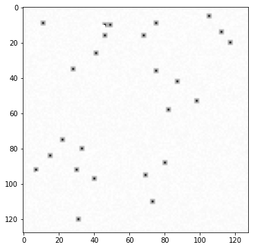
We can check the best sources extracted.

img.best_sources[['x', 'y', 'cflux']]

array([(74.99950543,  8.9952085 , 269.88079834),
       (46.00495959, 16.00276395, 268.41549683),
       (67.99847428, 16.00627683, 269.9263916 ),
       (40.99845109, 25.99984788, 268.90808105),
       (28.00398889, 34.99543308, 267.75750732),
       (75.00020406, 36.00161855, 267.00131226),
       (86.99742868, 42.00051015, 268.46685791),
       (98.00059635, 53.01035352, 267.27404785),
       (81.99934787, 58.00604355, 269.30249023),
       (21.99991067, 74.99746784, 268.52197266),
       (32.999547  , 80.00032554, 267.3571167 ),
       (15.00032772, 84.00220434, 268.28329468),
       (80.00352989, 88.00013903, 266.56143188),
       ( 6.99951973, 92.00160289, 265.66516113),
       (30.0013353 , 91.99455509, 266.05792236),
       (40.00159237, 97.00203221, 266.15142822)],
      dtype={'names':['x','y','cflux'], 'formats':['<f8','<f8','<f8'], 'offsets':[56,64,168], 'itemsize':240})

And also obtain the estimation of PSF.

As the PSF may vary across the field, we use the method described in Lauer T. (2002) for spatially variant PSF.

The methodology returns a series of image-sized coefficients \(a_i\) and a series of basis PSF elements \(p_i\).

a_fields, psf_basis = img.get_variable_psf()

updating stamp shape to (15,15)
(16, 16) (225, 16)

As in our simple example we don’t vary the PSF we obtain only a PSF element, and a None coefficient.

len(psf_basis), psf_basis[0].shape

(1, (15, 15))

a_fields

[None]

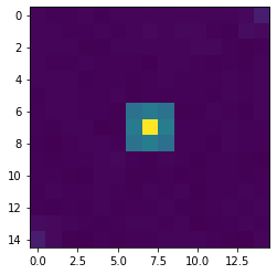
We may check the looks of the psf_basis single element.

plt.imshow(psf_basis[0])

<matplotlib.image.AxesImage at 0x7f6d00a85a90>