Tutorial - Part #2 - Spatially variant PSF
Introduction
This package hosts a simple implementation of the proposed technique by Lauer 2002.
The technique performs a linear decomposition of the PSF into several basis elements of small size (much smaller than the image) normalized to unit sum. Each of these autopsfs come with a coefficient, which is not normalized, that have the same size of the image.
To perform the decomposition uses the Karhunen-Loeve transform, in order to calculate the basis as a linear expansion of the psf observations –which are cutout stamps of the stars in the image.
[1]:
import numpy as np
import matplotlib.pyplot as plt

%matplotlib inline
[2]:
from properimage import simtools
from properimage import single_image as si
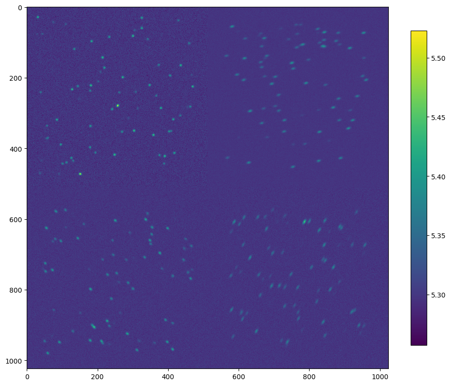
We simulate an image with several star shapes across the field
[3]:
frames = []
for theta in [0, 45, 105, 150]:
    N = 512  # side
    X_FWHM = 5 + 6.5*theta/180
    Y_FWHM = 5
    t_exp = 5
    max_fw = max(X_FWHM, Y_FWHM)
    #test_dir = os.path.abspath('./test/test_images/psf_basis_kl_gs')

    x = np.random.randint(low=6*max_fw, high=N-6*max_fw, size=80)
    y = np.random.randint(low=6*max_fw, high=N-6*max_fw, size=80)
    xy = [(x[i], y[i]) for i in range(80)]

    SN =  30. # SN para poder medir psf
    weights = list(np.linspace(10, 1000., len(xy)))
    m = simtools.delta_point(N, center=False, xy=xy, weights=weights)
    im = simtools.image(m, N, t_exp, X_FWHM, Y_FWHM=Y_FWHM, theta=theta,
                        SN=SN, bkg_pdf='gaussian')
    frames.append(im+100.)
[4]:
frame = np.zeros((1024, 1024))
for j in range(2):
    for i in range(2):
        frame[i*512:(i+1)*512, j*512:(j+1)*512] = frames[i+2*j]
[5]:
plt.figure(figsize=(12, 12))
plt.imshow(np.log(frame), interpolation='none')
plt.colorbar(shrink=0.7)
[5]:
<matplotlib.colorbar.Colorbar at 0x1372eecf0>
We perform the psf extraction.
This is possible to do with a context manager, in order to autoclean the disk files where the star stamps are stored.
[6]:
%%time

with si.SingleImage(frame, smooth_psf=False) as sim:
    a_fields, psf_basis = sim.get_variable_psf(inf_loss=0.15)
    x, y = sim.get_afield_domain()
updating stamp shape to (23,23)
CPU times: user 242 ms, sys: 52.5 ms, total: 295 ms
Wall time: 326 ms
[7]:
print(len(psf_basis))
4
This is equivalent to do the following:
[8]:
sim = si.SingleImage(frame, smooth_psf=False)
a_fields, psf_basis = sim.get_variable_psf(inf_loss=0.15)
x, y = sim.get_afield_domain()
updating stamp shape to (23,23)
In this case, we will have the sim object in memory and we need to close it to erase the auxiliary files being generated.
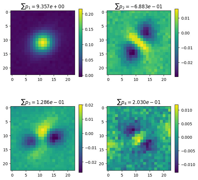
We can peek into the variable PSF
The autopsf elements are small patches, like the ones below.
The principal component psf is the first element of this list of arrays.
[9]:
ax = sim.plot.autopsf()
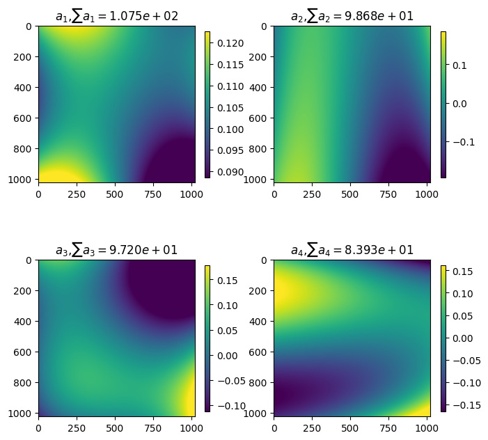
We can also plot the coefficients, they look as smooth fields of the same size of the image.
Whenever they grow they show where the corresponding autopsf element is more important than others.
[10]:
ax = sim.plot.autopsf_coef()
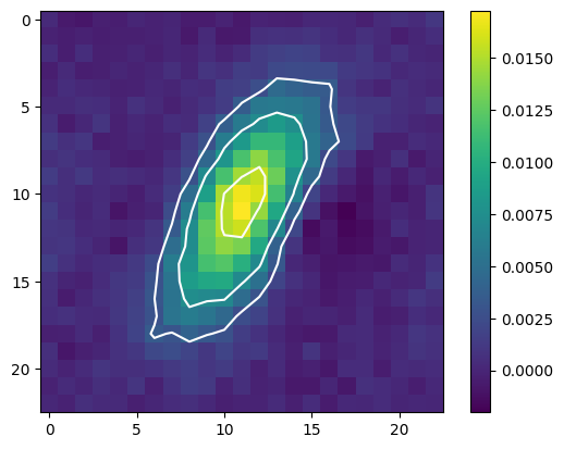
Rebuilding an image frame
In order to obtain the PSF value on any place of the image, we need to perform the summation of the autopsf elements weighted by the afields in the particular position we may desire.
[11]:
loc = (880, 995)

PSF_loc = np.zeros_like(psf_basis[0])
for apsf, afield in zip(psf_basis, a_fields):
    PSF_loc += apsf * afield(*loc)
[12]:
levels = np.logspace(-2.5, -0.5, num=7)

plt.imshow(PSF_loc)
plt.colorbar()
plt.contour(PSF_loc, levels=levels, cmap='Greys')
[12]:
<matplotlib.contour.QuadContourSet at 0x107ae34d0>
[13]:
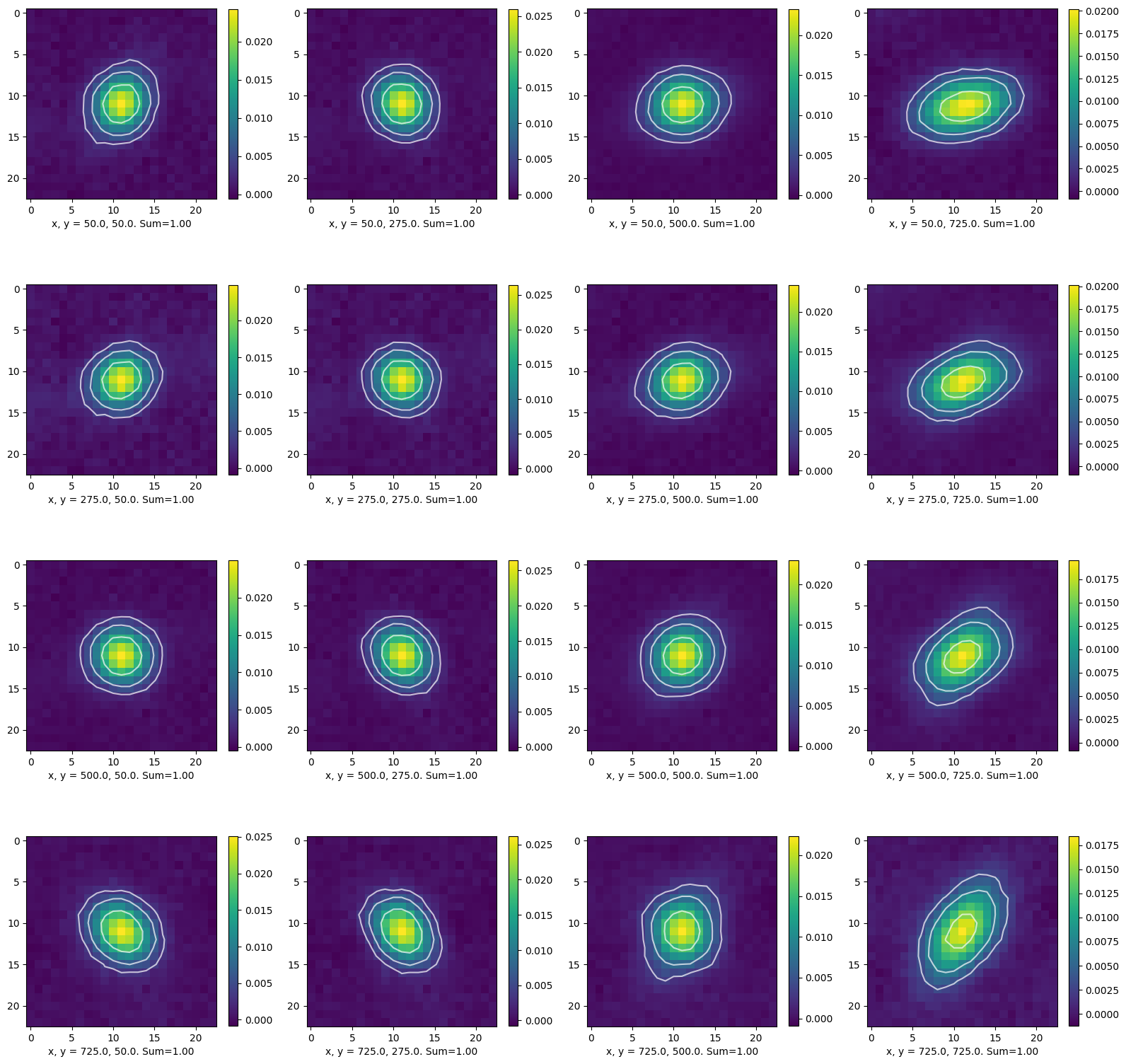
xs = np.repeat(np.arange(50, 950, 900/4), 4)
ys = np.array([np.repeat(50+i*900/4., 4) for i in range(4)]).T.flatten()

i = 0
plt.figure(figsize=(16, 16))
for xp, yp in zip(xs, ys):
    PSF_loc = sim.get_psf_xy(xp, yp)
    plt.subplot(4, 4, i+1)
    plt.imshow(PSF_loc/np.sum(PSF_loc))
    plt.colorbar(shrink=0.7)
    plt.contour(PSF_loc, cmap='Greys', alpha=0.7, levels=levels)
    plt.xlabel(f'x, y = {np.round(xp)}, {np.round(yp)}. Sum={np.sum(PSF_loc):.2f}')
    i += 1
plt.tight_layout()
[ ]: