Tutorial - Part #3 - Advanced SingleImage
In this tutorial a more advanced set of examples are presented on SingleImage class, which allows tod do more specific tasks with the instances.
We import the packages, and also a pair of sample images
[1]:
import numpy as np
import matplotlib.pyplot as plt
%matplotlib inline
[2]:
from astropy.visualization import LinearStretch, LogStretch, ZScaleInterval, MinMaxInterval, ImageNormalize
[3]:
import properimage.single_image as si
[4]:
img_path = './../../../data/aligned_eso085-030-004.fit'
[5]:
img = si.SingleImage(img_path)
Quickly we get the answer for the number of sources a priori we would use and the estimated size of thw PSF cutout stamp.
If we want to know the different properties assigned to this instance we can enumerate them:
The origin of the information:
[6]:
print(img.attached_to)
./../../../data/aligned_eso085-030-004.fit
The header if a fits file
[7]:
img.header
[7]:
SIMPLE  =                    T / conforms to FITS standard
BITPIX  =                   16 / array data type
NAXIS   =                    2 / number of array dimensions
NAXIS1  =                 1024
NAXIS2  =                  682
DATE-OBS= '2015-12-27T06:26:24' /YYYY-MM-DDThh:mm:ss observation start, UT
EXPTIME =   60.000000000000000 /Exposure time in seconds
EXPOSURE=   60.000000000000000 /Exposure time in seconds
SET-TEMP=  -20.000000000000000 /CCD temperature setpoint in C
CCD-TEMP=  -20.091654000000002 /CCD temperature at start of exposure in C
XPIXSZ  =   27.000000000000000 /Pixel Width in microns (after binning)
YPIXSZ  =   27.000000000000000 /Pixel Height in microns (after binning)
XBINNING=                    3 /Binning factor in width
YBINNING=                    3 /Binning factor in height
XORGSUBF=                    0 /Subframe X position in binned pixels
YORGSUBF=                    0 /Subframe Y position in binned pixels
READOUTM= 'Monochrome (Preflash)' /Readout mode of image
FILTER  = 'Clear   ' /          Filter used when taking image
IMAGETYP= 'Light Frame' /       Type of image
SITELAT = '-31 35 48' /         Latitude of the imaging location
SITELONG= '-64 32 56' /         Longitude of the imaging location
JD      =   2457383.7683333335 /Julian Date at start of exposure
FOCALLEN=   7475.0000000000000 /Focal length of telescope in mm
APTDIA  =   1540.0000000000000 /Aperture diameter of telescope in mm
APTAREA =   1862650.3361463547 /Aperture area of telescope in mm^2
SWCREATE= 'MaxIm DL Version 5.24 130605 0QTH7' /Name of software that created
         the image
SBSTDVER= 'SBFITSEXT Version 1.0' /Version of SBFITSEXT standard in effect
OBJECT  = 'eso085-030'
TELESCOP= '        ' /          telescope used to acquire this image
INSTRUME= 'Apogee USB/Net'
OBSERVER= '        '
NOTES   = '        '
FLIPSTAT= '        '
SWOWNER = 'Mario C Diaz' /      Licensed owner of software
BSCALE  =                    1
BZERO   =                32768
COMMENT aligned img /home/bruno/Documentos/Data/ESO085-030/eso085-030-004.fit to
COMMENT  /home/bruno/Documentos/Data/ESO085-030/eso085-030-003.fit
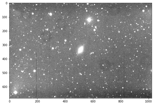
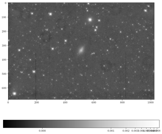
The pixel data
[8]:
norm = ImageNormalize(img.data, interval=ZScaleInterval(),
                      stretch=LinearStretch())

plt.figure(figsize=(9,10))
plt.imshow(img.data, cmap='Greys_r', norm=norm)
[8]:
<matplotlib.image.AxesImage at 0x118935550>
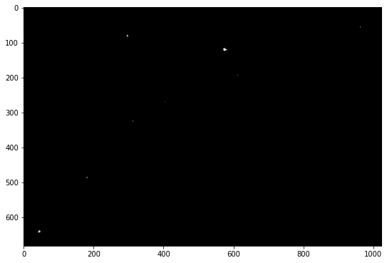
The mask inferred or setted
[9]:
plt.figure(figsize=(9,10))
plt.imshow(img.mask, cmap='Greys_r')
[9]:
<matplotlib.image.AxesImage at 0x119eb0910>
The background calculated
[10]:
plt.figure(figsize=(9,10))
plt.imshow(img.background, cmap='Greys_r')
plt.colorbar(orientation='horizontal')
plt.tight_layout()
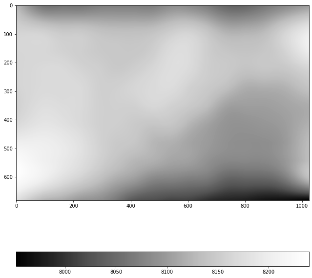
As the background is being estimated only if accesed, then it prints the results.
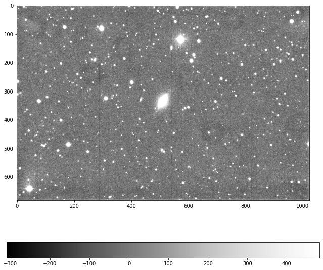
The background subtracted image
[11]:
norm = ImageNormalize(img.bkg_sub_img, interval=ZScaleInterval(),
                      stretch=LinearStretch())
plt.figure(figsize=(9,8))
plt.imshow(img.bkg_sub_img, cmap='Greys_r', norm=norm)
plt.colorbar(orientation='horizontal')
plt.tight_layout()
It also can be obtained a interpolated version of this image. The interpolated version is replacing masked pixels by using a box kernel convolutional interpolation:
[12]:
norm = ImageNormalize(img.bkg_sub_img, interval=ZScaleInterval(),
                      stretch=LinearStretch())
plt.figure(figsize=(9,8))
plt.imshow(img.interped, cmap='Greys_r', norm=norm)
plt.colorbar(orientation='horizontal')
plt.tight_layout()

The stamp_shape to use (this is the final figure, after some exploring of the stars chosen)
[13]:
print(img.stamp_shape)
(15, 15)
Get the stamp positions is also possible
[14]:
print(img.stamps_pos[0:10])
updating stamp shape to (21,21)
[[  4.00943643  25.26128594]
 [  7.14687061 480.90912976]
 [ 11.72773176 610.83903618]
 [ 12.82933208 193.25984595]
 [ 19.53524876 493.70670392]
 [ 41.55364625 548.48252311]
 [ 50.58756504  31.54122567]
 [ 64.95489806 704.69765379]
 [ 70.30182444 373.69091315]
 [ 74.96856997 282.51691302]]
Obtaining the best sources was explained in Tutorial 01, but here we show it again just to be complete
[15]:
print(img.best_sources[0:10][['x', 'y', 'cflux']])
[( 25.26128594,  4.00943643, 53946.6875    )
 (480.90912976,  7.14687061, 24435.078125  )
 (610.83903618, 11.72773176, 40933.87109375)
 (193.25984595, 12.82933208, 47999.0546875 )
 (493.70670392, 19.53524876, 30155.66015625)
 (548.48252311, 41.55364625, 48258.04296875)
 ( 31.54122567, 50.58756504, 22010.3984375 )
 (704.69765379, 64.95489806, 18889.390625  )
 (373.69091315, 70.30182444, 19581.18359375)
 (282.51691302, 74.96856997, 24461.18359375)]
We can get the final number of sources used in PSF estimation
[16]:
print(img.n_sources)
83
We can also print the covariance matrix from these objects
[17]:
print(img.cov_matrix)
[[8.98636326e-05 6.08960412e-05 7.32952701e-05 ... 5.38147805e-05
  5.81110432e-05 8.01231966e-05]
 [6.08960412e-05 5.48571430e-05 5.77536897e-05 ... 4.10838639e-05
  4.41064959e-05 5.80219676e-05]
 [7.32952701e-05 5.77536897e-05 7.42381796e-05 ... 4.84207302e-05
  5.77348556e-05 7.41418902e-05]
 ...
 [5.38147805e-05 4.10838639e-05 4.84207302e-05 ... 4.25014802e-05
  3.73796658e-05 5.00585935e-05]
 [5.81110432e-05 4.41064959e-05 5.77348556e-05 ... 3.73796658e-05
  5.33515884e-05 6.23979798e-05]
 [8.01231966e-05 5.80219676e-05 7.41418902e-05 ... 5.00585935e-05
  6.23979798e-05 9.33261254e-05]]
As showed from Tutorial 02 we can get the PSF, depending on our level of approximation needed
[18]:
a_fields, psf_basis = img.get_variable_psf(inf_loss=0.01)
[19]:
print(len(psf_basis), len(a_fields))
46 46
Check the information loss argument, which states the maximum amount of information lost in the basis expansion. If we change it the basis is updated:
[20]:
a_fields, psf_basis = img.get_variable_psf(inf_loss=0.10)
print(len(psf_basis), len(a_fields))
3 3
Of course the elements of the basis are unchanged, only a subset is returned. So going from small inf_loss to bigger values is the same as choosing less elements in the calculated basis.
Once obtained this basis and coefficient fields we can display them using some of the builtin plot functionalities:
[21]:
axs = img.plot.autopsf()

For the a_fields object we used to need to give the coordinates where we would evaluate this coefficients. That function is still provided, inside img instance object.
[22]:
x, y = img.get_afield_domain()
However, the plot plugin attribute contains a plotting method that already handles that.
[23]:
axs = img.plot.autopsf_coef()

The instance is capable of calculating its own \(S\) component (Zackay et al. 2016 notation)
[24]:
S = img.s_component
[25]:
norm = ImageNormalize(S, interval=MinMaxInterval(),
                      stretch=LogStretch())
plt.figure(figsize=(9,8))
plt.imshow(S, cmap='Greys_r', norm=norm)
plt.colorbar(orientation='horizontal')
plt.tight_layout()
We can also attempt to place our PSF measurement on top of the stars of the image. This is done by placing a delta function in each star position, and convolving with the autopsfs obtained, and add them weighted with the a(x,y) fields.
[26]:
a_fields, psf_basis = img.get_variable_psf(inf_loss=0.05)
[27]:
plt.figure(figsize=(12, 6))
for i in range(8):
    nsrc = np.random.randint(0, img.n_sources)
    xc, yc = img.best_sources[nsrc][['y', 'x']]
    try:
        patch = si.extract_array(img.data, img.stamp_shape,
                                 [xc, yc], fill_value=img._bkg.globalrms, mode='strict')
    except:
        nsrc = np.random.randint(0, img.n_sources)
        xc, yc = img.best_sources[nsrc][['y', 'x']]
        patch = si.extract_array(img.data, img.stamp_shape,
                                 [xc, yc], fill_value=img._bkg.globalrms, mode='strict')

    plt.subplot(2, 4, i+1)
    patch = np.log10(patch)
    plt.imshow(patch, vmin=np.percentile(patch, q=10), vmax=np.percentile(patch, q=98))
    plt.tick_params(labelsize=16)
    try:
        thepsf = img.get_psf_xy(xc, yc)
    except ValueError:
        print(xc, yc)
    #print(patch.shape, thepsf.shape)
    labels = {'sum': np.sum(thepsf)}
    plt.title(r'$\sum PSF = {sum:4.3f}$'.format(**labels))
    plt.contour(thepsf, levels=[0.0015, 0.003, 0.01, 0.03], cmap='Greys')

plt.tight_layout()
/Users/sanchez/.virtualenvs/dev2026/lib/python3.13/site-packages/numpy/lib/_function_base_impl.py:4859: UserWarning: Warning: 'partition' will ignore the 'mask' of the MaskedArray.
  arr.partition(

[ ]: